


In this article, we aim to discuss various GLMs that are widely used in the industry. We focus on: a) log-linear regression b) interpreting log-transformations and c) binary logistic regression.
Editor’s note:Data files discussed below can be acquired here:
Generalized Linear Model (GLM) helps represent the dependent variable as a linear combination of independent variables. Simple linear regression is the traditional form of GLM. Simple linear regression works well when the dependent variable is normally distributed. The assumption of normally distributed dependent variable is often violated in real situations. For example, consider a case where dependent variable can take only positive values and has fat tail. The dependent variable is number of coffee sold and the independent variable is the temperature.
Let’s assume that we have modeled a linear relationship between the variables. The expected number of coffee sold decreases by 10 units as temperature increases by 1 degree. The problem with this kind of model is that it can give meaningless results. There will be situation when a increase of 1 degree in temperature would force the model to output negative number for number of coffee sold. GLM comes in handy in these types of situations. GLM is widely used to model situations where the independent variable has arbitrary distributions i.e. distributions other than normal distribution. The basic intuition behind GLM is to not model dependent variable as a linear combination of independent variable but model a function of dependent variable as a linear combination of dependent variable. This function used to transform independent variable is known as link function. In the above example the distribution of number of coffee sold will not be normal but poisson and the log transformation (log will be the link function in this case) of the variable before regression would lead to a logical model. The ability of GLM to transform data with arbitrary distribution to fit a meaningful linear model makes it a powerful tool.
In this article, we aim to discuss various GLMs that are widely used in the industry. We focus on: a) log-linear regression b) interpreting log-transformations and c) binary logistic regression. We also review the underlying distributions and the applicable link functions. However, we start the article with a brief discussion on the traditional form of GLM, simple linear regression. Along with the detailed explanation of the above model, we provide the steps and the commented R script to implement the modeling technique on R statistical software. For the purpose of illustration on R, we use sample datasets. We hope that you find the article useful.
Linear Regression
Linear regression is the most basic form of GLM. Linear regression models a linear relationship between the dependent variable, without any transformation, and the independent variable. The model assumes that the variables are normally distributed. It is represent in the form Yi= α+ βXi [Eq. 1]. The coefficients are computed using the Ordinary Least Square (OLS) method. For a detailed explanation on linear regression and OLS, please refer to our earlier article at building regression models support vector regression. The article provides explanation and an example of linear regression. We hope that now you are comfortable with the idea of linear regression.
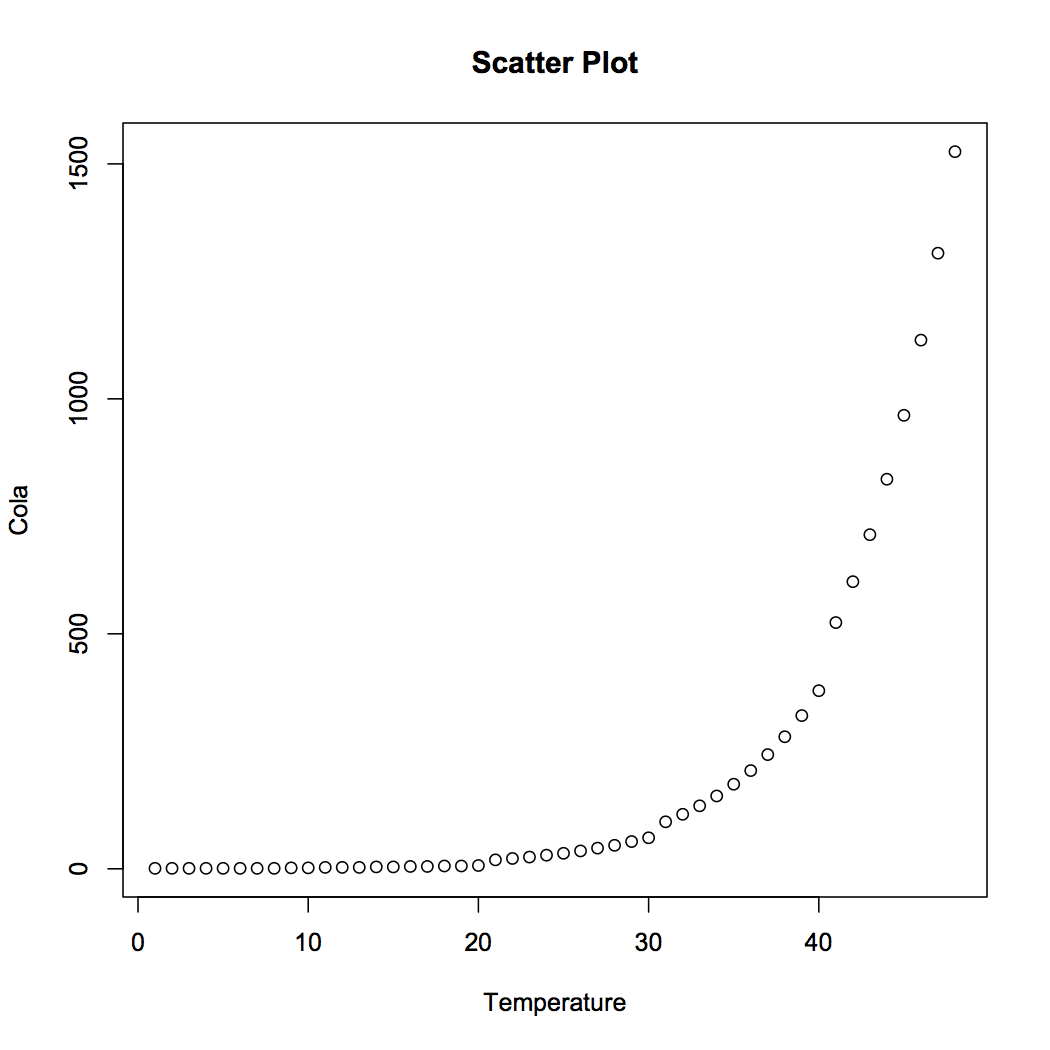
Now, with the objective of showing limitation of linear regression, we will implement the linear model on R using a not so perfect case. The data consists of two variables – Temperature and Coca-Cola sales in a university campus. Please click here to download. Let us visualize the data and fit a linear model to predict sales of coca cola based on given temperature.
The R code is below:
## Prepare scatter plot

#Read data from .csv file
data = read.csv("Cola.csv", header = T)
head(data)

#Scatter Plot
plot(data, main = "Scatter Plot")
## Add best-fit line to the scatter plot
#Install Package
install.packages("hydroGOF")
library("hydroGOF")
#Fit linear model using OLS
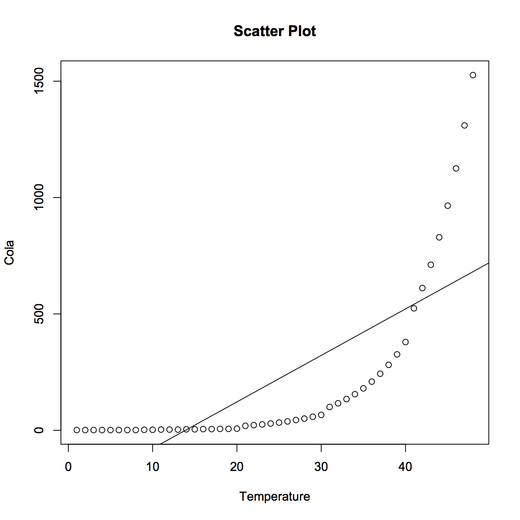
model = lm(Cola ~ Temperature, data)
#Overlay best-fit line on scatter plot
abline(model)
#Calculate RMSE
PredCola = predict(model, data)
RMSE = rmse(PredCola, data$Cola)
The relationship between Temperature and Cola Sales is represented in Equation [2]. The Root Mean Square Error for the model is pretty high at 241.49. The values of cola sales can be obtained by plugging the temperature in the equation.
 [2]
[2]
Log-Linear Regression
Log-linear regression becomes a useful tool when the dependent and independent variable follow an exponential relationship. It means that Y does not change linearly with a unit change in X but Y changes by a constant percentage with unit change in X. For example, the amount due, in case of compound interest, follows an exponential relationship with time, T. As T increases by one unit, the amount due increases by a certain percentage i.e. interest rate. Another example can be that of expected salary and education. Expected salary does not follow a linear relationship with level of education. It grows exponentially with level of education. Such growth models depict a variety of real life situations and can be modeled using log-linear regression. Apart from exponential relationship, log transformation on dependent variable is also used when dependent variable follows: a) log-normal distribution – log-normal distribution is distribution of a random variable whose log follows normal distribution. Thus, taking log of a log-normal random variable makes the variable normally distributed and fit for linear regression. b) Poisson distribution – Poisson distribution is the distribution of random variable that results from a Poisson experiment. For example, the number of successes or failures in a time period T follows Poisson distribution.
In this article we focus on the exponential relationship, which is expressed asY=a(b)X[Eq. 2]. In this case, a log transformation would make the relationship linear. We can representlog(Y)as a linear combination on Xs. Taking log on both sides in the equation, we get log(Y)=log(a)+log(b)X. Now we can estimate the model using OLS. Please note that this equation is very similar to Eq. 1,log(a)andlog(b)are equivalent toαandβrespectively. Now we will look into interpretation of log linear models.log(a)is the constant term andlog(b)is the growth rate with which Y grows for a unit change in X. A negative value oflog(b)would indicate that Y decreases by a certain percentage for unit increase in X. Now we will implement the model on R using the Coca-Cola sales data.
The R code is below.
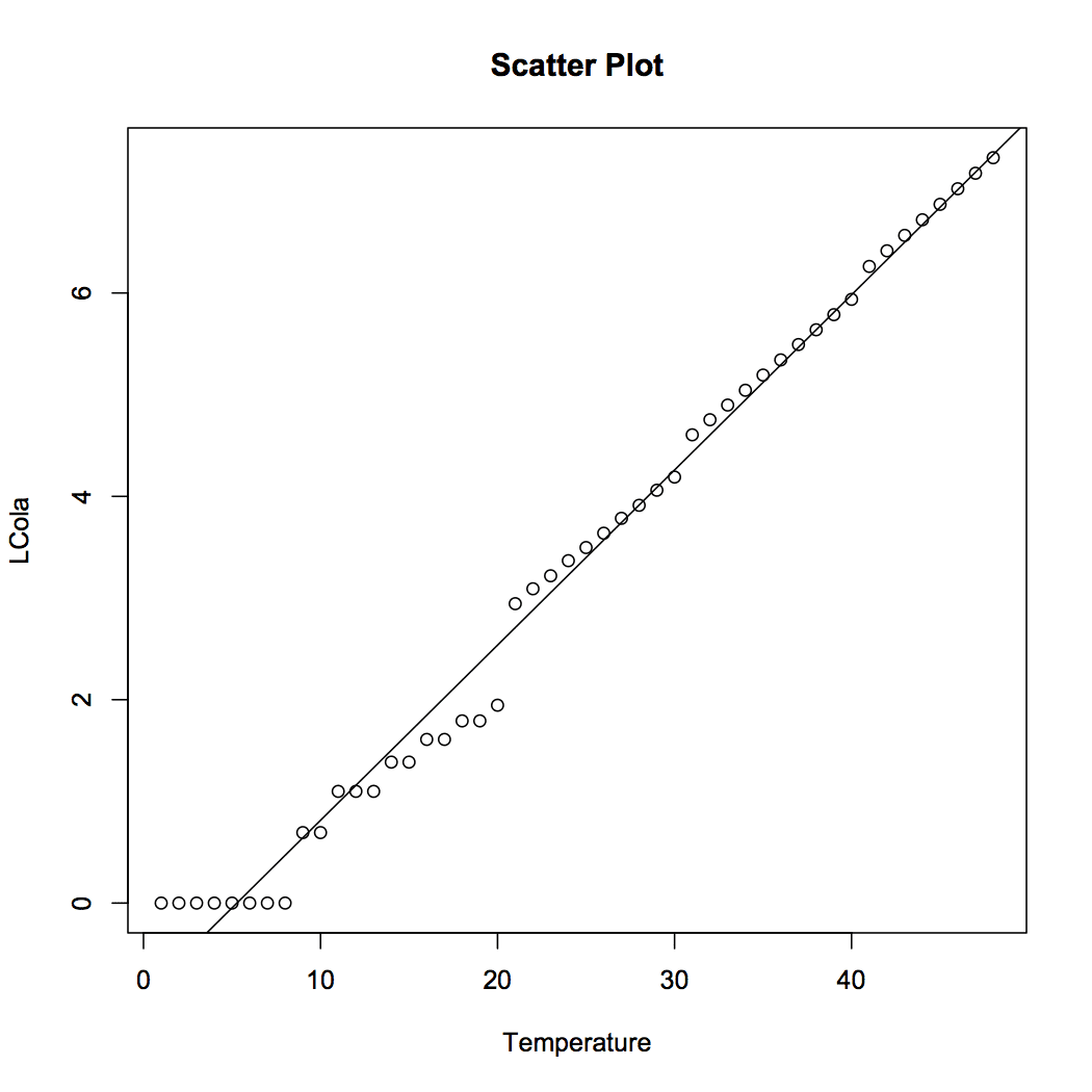
## Fitting Log-linear model

# Transform the dependent variable
data$LCola = log(data$Cola, base = exp(1))

#Scatter Plot
plot(LCola ~ Temperature, data  = data , main = "Scatter Plot")

#Fit the best line in log-linear model
model1 = lm(LCola ~ Temperature, data)
abline(model1)

#Calculate RMSE
PredCola1 = predict(model1, data)
RMSE = rmse(PredCola1, data$LCola)
 [3]
[3]
The Cola sales can be predicted by plugging the values of temperature in Equation [3]. We observe that the fit has greatly improved over the simple linear regression. The RMSE for the transformed model is 0.24 only. Please note that log-linear regression has also solved the issue of absurd negative values for cola sales. For no value of temperature we get a negative value of cola sales. A simple log transformation helps us to deal with the absurdity. In the next section we will discuss other log transformations that come handy in various situations.
Interpreting Log Transformations
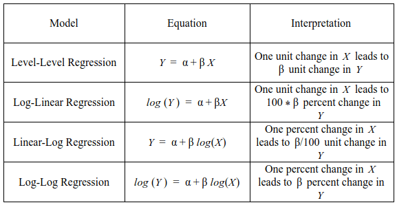
Log transformations of dependent and independent data is an easy way to handle non-linear relationships. The transformation helps to analyze non-linear relationships using linear models. We have discussed the log-linear regression. There are two more variants – a) linear–log regression –the independent variables are log transformed and b) log-log regression – both the dependent and independent variables are transformed. The table below displays the equations and interpretation for each of the models.
Binary Logistic Regression
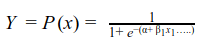
Binary logistic regression is used when the dependent variable is categorical and takes values – 0 and 1. Unlike simple linear regression, where conditional distribution of dependent variable is normal, in logistic regression the conditional distribution of dependent variable is Bernoulli. In Bernoulli distribution the variable can only take two values – 0 and 1 with certain probabilities.
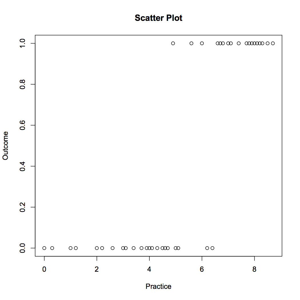
Lets understand with the help of an example. Let us assume that in football the ability to convert a penalty depends on number of hours of practice by the shooter. We can represent a successful penalty by 1 and an unsuccessful penalty by 0. The data looks as follows:

 [4]
[4]
A positive value (negative value) of β1 would indicate that probability of Y=1 increases (decreases) as X increases. Logistic regression is one of the widely used model of class prediction. The multinomial logistic regression extends the binary model to deal with problems involving multiple classes. For example, whether a person will redeem coupon A, coupon B or coupon C. Now we will implement the logistic regression model in R. The sample data consists of two variables – success/ failure in penalty shoot out represent 1/0 and hours of practice.
The R code is follows:
## Prepare scatter plot

#Read data from .csv file
data1 = read.csv("Penalty.csv", header = T)
head(data1)

#Scatter Plot
plot(data1, main = "Scatter Plot")
The R code is as follows:
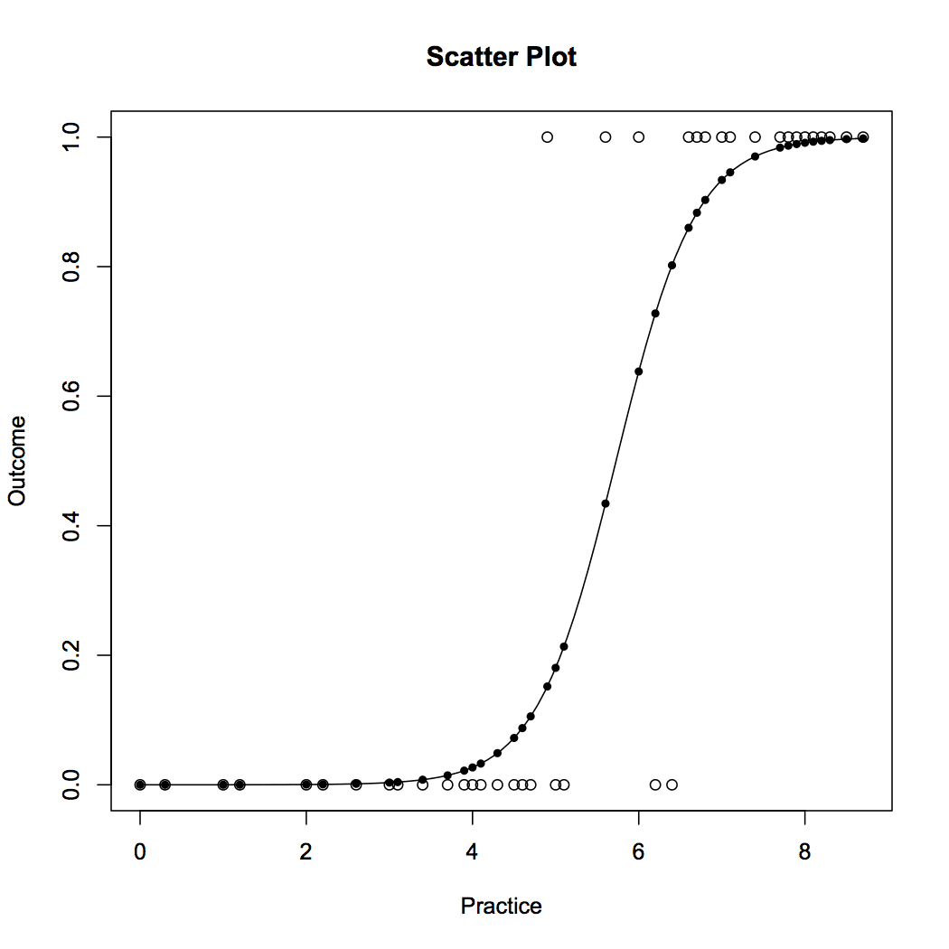
## Fitting Logistic regression model
fit = glm(Outcome ~ Practice, family = binomial(link = "logit"), data = data1)

#Plot probabilities
plot(data1, main ="Scatter Plot")
curve(predict(fit,data.frame(Practice = x), type = "resp"), add = TRUE)
points(data1$Practice,fitted(fit),pch=20)
Figure 5 displays the probability values obtained from the logistic regression. We can see that the model does a good job. The probability of success increases with increase in practice hours. The model is represented in equation [5]. The probability values can be obtained by plugging in the number of practice hours.
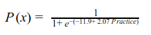 [5]
[5]
Conclusion
In this article we learned about Generalized Linear Model (GLM). Simple linear regression is the most basic form of GLM. Advance form of GLM helps to deal with non-normal distributions and non-linear relationships in a simple manner. We focus on log-linear regression and binary logistic regression. Log-linear regression is useful when the relation between dependent and independent variable is non-linear. It also provides a quick fix when dependent variable follows log-normal or Poisson distribution.
Further, we discussed the basic concepts of binary logistic regression. Binary logistic regression is beneficial when the dependent variable follows Bernoulli distribution, i.e. can take only values of 0 and 1. We also provide equations and interpretation for various log transformations that are used with regression models.
Along with the theoretical explanation, we share the R codes, so that you can implement the model on R. For better understanding, we display the results along with the codes.
We hope you find the article is useful.
Looking to do more with your data? Check out our other services : Power BI Consulting | Power BI Expert | Power BI Consultant | Tableau Consultants | Tableau Consulting | Tableau Expert | Tableau Contractor | Tableau Freelance Developer | Tableau Developer